Thermal metamaterial (2D)#
In this example, we design a metamaterial with effective thermal conductivity
where \(\kappa_{xx} = \kappa_{yy} = 0.2 \ \text{W}\cdot\text{m}^{-1}\cdot\text{K}^{-1}\) and \(\kappa_{xy} = \kappa_{yx} = -0.05 \ \text{W}\cdot\text{m}^{-1}\cdot\text{K}^{-1}\).
The thermal conductivity along a given direction \(\hat{\mathbf{n}}\) is given by
We solve the heat conduction for the directions \(\hat{\mathbf{n}}_0 = \hat{\mathbf{x}}\), \(\hat{\mathbf{n}}_1 = \hat{\mathbf{y}}\), and \(\hat{\mathbf{n}}_2 = \frac{\sqrt{2}}{2} \hat{\mathbf{x}} + \frac{\sqrt{2}}{2} \hat{\mathbf{y}}\), leading to the linear system
Density-based topology optimization is performed using the three-field approach, as outlined here for thermal materials.
Notes:
We use the recently introduced subpixel smoothed projection.
We specify
batch_size=3when creating theFourierobject.With
collapse_direct=True, we use the same matrix assembly for each direction, which is more efficient. This option is only available for the direct solver.
from matinverse import Geometry2D,BoundaryConditions,Fourier
from matinverse.projection import projection
from matinverse import Movie2D,Plot2D
from matinverse.filtering import Conic2D
from matinverse.optimizer import MMA,State
from jax import numpy as jnp
from functools import partial
import jax
L = 10
size = [L,L]
N = 100
grid = [N,N]
geo = Geometry2D(grid,size,periodic=[True,True]) #
Ainv = jnp.array([[1,0,0],[0,1,0],[-0.5,-0.5,1]])
phi = jnp.array([0,jnp.pi/2,jnp.pi/4])
directions = jnp.array([jnp.cos(phi),jnp.sin(phi)]).T
bcs = BoundaryConditions(geo)
bcs.periodic('x',lambda batch,space,t:directions[batch,0])
bcs.periodic('y',lambda batch,space,t:directions[batch,1])
kappa_bulk = jnp.eye(2)
kd = jnp.array([0.2,0.3,-0.05])
delta = 1e-12
R = L/10
filtering = Conic2D(geo,R)
def transform(x,beta):
x = filtering(x)
return projection(x,beta=beta,resolution=N/L)
@jax.jit
def objective(rho,beta):
rho = transform(rho,beta)
rho = delta + rho*(1-delta)
kappa_map = lambda batch,space,temp,t: kappa_bulk*rho[space]
out = Fourier(geo,bcs,kappa_map,batch_size=3,linear_solver='direct',collapse_direct='True')[0]
out['projected_rho'] = rho
kappa_effective = jnp.matmul(Ainv,out['kappa_effective'])
g = jnp.linalg.norm(kappa_effective-kd)
return g,({'kappa':kappa_effective},out)
betas = [8,16,jnp.inf]
maxiter = [20,20,40]
state = State()
x = jax.random.uniform(jax.random.PRNGKey(1), N**2)
for k,beta in enumerate(betas):
print(beta)
x= MMA( partial(objective,beta=beta), \
x0=x,\
state = state,\
nDOFs = N**2,\
maxiter=maxiter[k])
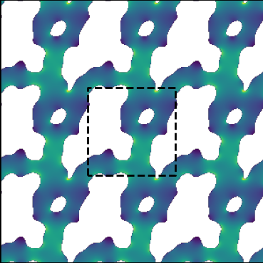
J = jnp.linalg.norm(state.aux[-1]['J'],axis=(0,2))
evolution = jnp.array([aux['projected_rho'] for aux in state.aux])
design_mask = x.reshape(grid)
Plot2D(J,geo,design_mask = design_mask ,cmap='viridis',write=True)
Movie2D(evolution,geo,cmap='binary')